Here is a persuasive advertisement for ghostwriting services for the topic of Fourier series:
**Get Expert Help with Your Fourier Series Assignments!**
Are you struggling to understand the complex concepts of Fourier series? Do you need help with your assignments, research papers, or projects on this topic?
Our team of expert ghostwriters specializes in providing high-quality writing services for students in mathematical physics and related fields. With our help, you can:
* Get a deep understanding of the origins of Fourier series, from the 1746 vibrating string problem to modern applications
* Master the mathematical techniques and concepts underlying Fourier series
* Produce well-researched and well-written assignments, papers, and projects that showcase your knowledge and skills
Our ghostwriting services include:
* Customized writing solutions tailored to your specific needs and requirements
* In-depth research and analysis of the topic, ensuring accuracy and relevance
* Clear and concise writing that effectively communicates complex ideas
* Timely delivery of your work, ensuring you meet your deadlines
Why choose our ghostwriting services?
* Expertise: Our writers have advanced degrees in mathematical physics and related fields, ensuring they have a deep understanding of the subject matter.
* Quality: We guarantee high-quality work that meets your expectations and exceeds your standards.
* Confidentiality: We maintain strict confidentiality and ensure that your work is kept private and secure.
Don’t let your Fourier series assignments hold you back any longer. Get expert help today and achieve academic success!
Order now and let us take care of your writing needs!
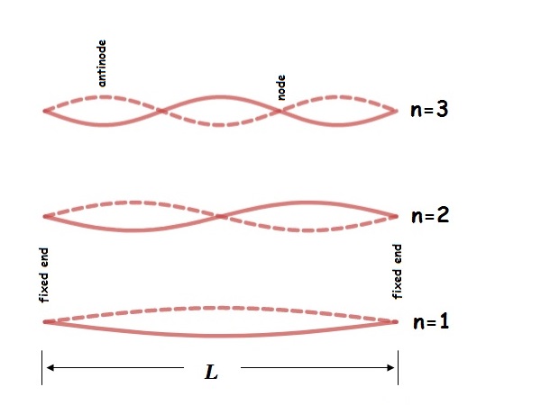
The theory of Fourier series has its roots in the problems of mathematical physics. The story begins in 1746 with a famous _vibrating string problem_. Consider an elastic string of length \(L\) which has each end fastened to one of the end points of the interval \([0,L]\) on the \(x\)-axis and set into motion (just like when you pluck a guitar string). The question is to determine the position \(y=F(x,t)\) of the string at a time \(t\) provided its initial position \(F(x,0)=f(x)\) and initial velocity \(F_{t}(x,0)=0\). The function \(F(x,t)\) is the solution of the so-called _d’Alembert’s wave equation_:
\[F_{tt}=a^{2}F_{xx},\]
where the initial data for this problem is
\[F(x,0)=f(x),\quad F_{t}(x,0)=0,\quad f(0)=0=f(L),\]
and \(a\) is a positive constant determined by the physical properties of the string. It is not hard to find particular solutions to the wave equation, for example each of the functions
\[F(x,t)=\sin\left(\frac{k\pi x}{L}\right)\cos\left(\frac{ak\pi t}{L}\right)\quad k =1,2,\ldots\]
[MISSING_PAGE_FAIL:235]
### Orthogonality Relations
The theory of Fourier series is based on orthogonality relations for sines and cosines. By analogy with the concept of orthogonal vectors in \(\mathbb{R}^{n}\), two functions \(f\) and \(g\) are said to be orthogonal over the interval \([a,b]\) if
\[\int_{a}^{b}f(x)\,g(x)\,dx=0.\]
Recalling the trigonometric identities
\[2\cos nx\sin mx=\sin(n+m)x-\sin(n-m)x,\]
\[2\cos nx\cos mx=\cos(n+m)x+\cos(n-m)x,\]
\[2\sin nx\sin mx=\cos(n-m)x-\cos(n+m)x,\]
it is not hard to see the following fundamental orthogonal relations:
\[\int_{-\pi}^{\pi}\cos nx\,dx=\int_{-\pi}^{\pi}\sin nx\,dx=0,\quad n=1,2,\dots,\]
\[\int_{-\pi}^{\pi}\cos nx\sin mx\,dx=0,\quad n,m=1,2,\dots,\]
\[\int_{-\pi}^{\pi}\cos nx\,\cos mx\,dx=\int_{-\pi}^{\pi}\sin nx\,\sin mx\,dx=0, \quad n\neq m,\]
\[\int_{-\pi}^{\pi}\cos^{2}nx\,dx=\int_{-\pi}^{\pi}\sin^{2}nx\,dx=\pi,\quad n=1, 2,\dots.\]
Suppose that for some coefficients \(a_{k}\) and \(b_{k}\) the trigonometric series
\[f(x)=\frac{a_{0}}{2}+\sum_{k=1}^{\infty}\left(a_{k}\cos kx+b_{k}\sin kx\right)\]
converges uniformly in the interval \([-\pi,\pi]\) to a sum \(f(x)\). Because we have uniform convergence, the function \(f\) is continuous and we can integrate this series term by term. Thus
\[\int_{-\pi}^{\pi}f(x)\,dx=\int_{-\pi}^{\pi}\frac{1}{2}a_{0}\,dx=\pi a_{0}.\]
Next, multiply \(f(x)\) by \(\cos nx\) for some index \(n=1,2,\dots\) and integrate term by term to find
\[\int_{-\pi}^{\pi}f(x)\,\cos nx\,dx = \sum_{k=1}^{\infty}a_{k}\int_{-\pi}^{\pi}\cos kx\cos nx\,dx+\sum_{ k=1}^{\infty}b_{k}\int_{-\pi}^{\pi}\sin kx\cos nx\,dx\] \[= \pi a_{n}+0=\pi a_{n}.\]These all follow from the orthogonality relations described above. Similarly, multiplication by \(\sin nx\) and integration gives
\[\int_{-\pi}^{\pi}f(x)\,\sin nx\,dx=\pi b_{n}.\]
**Definition 82**.: The Fourier series of the \(2\pi\) periodic function \(f:[-\pi,\pi]\to\mathbb{R}\) which is bounded and Riemann integrable on \([-\pi,\pi]\) is given by
\[f(x)=\frac{a_{0}}{2}+\sum_{k=1}^{\infty}\left(a_{k}\cos kx+b_{k}\sin kx\right),\]
where
\[a_{0}=\frac{1}{2}\int_{-\pi}^{\pi}f(x)\,dx\]
and
\[a_{n}=\frac{1}{\pi}\int_{-\pi}^{\pi}f(x)\,\cos nx\,dx,\quad n=0,1,2,\ldots\]
\[b_{n}=\frac{1}{\pi}\int_{-\pi}^{\pi}f(x)\,\sin nx\,dx,\quad n=1,2,\ldots.\]
The coefficients \(a_{n}\) and \(b_{n}\) are called the Fourier coefficients of \(f\) (or amplitudes) for the Fourier series.
Clearly, such a definition can be applied to those functions for which the above integrals exist. The point here, as we will see, is that most functions are actually equal to their Fourier series. Fourier’s work, even though considered by his contemporaries to be clumsy and non-rigorous, contains a real innovation. He transformed the existence of a series representation into a geometrically obvious fact that the area bounded by \(y=f(x)\,\sin mx\) and the \(x\)-axis between \(x=-\pi\) and \(x=\pi\) can always be computed. In other words he claimed that the Fourier coefficients of an arbitrary bounded function could always be determined.
**Example 87**.: In calculating Fourier coefficients of a given function \(f\), it is useful to take advantage of special symmetries. For example, if \(f\) is an even function, then \(f(x)\sin nx\) is odd, then it is clear without calculation that Fourier sine coefficients of \(f\) must vanish; in other words \(b_{n}=0\) for all \(n\). Similarly, if \(f\) is an odd function, or if it differs by a constant from an odd function, then \(a_{n}=0\) for all \(n\geq 1\) and the formula for \(b_{n}\) may be simplified. Now, we find the Fourier coefficients of the following functions.
* Let \(f(x)=x^{2}\). Since \(f(-x)=f(x)\) this is an even function and its Fourier series reduces to \[x^{2}=\sum_{n=1}^{\infty}a_{n}\cos nx.\]To get the Fourier coefficients we consider the following integrals and apply integration by parts to obtain: \[a_{n}=\frac{1}{\pi}\int_{-\pi}^{\pi}x^{2}\,\cos nx\,dx=\frac{4}{n^{2}}(-1)^{n} \quad n>0,\] \[a_{0}=\frac{1}{\pi}\int_{-\pi}^{\pi}x^{2}\,dx=\frac{2\pi^{2}}{3}.\] Thus, the function \(f(x)=x^{2}\) in the interval \([-\pi,\pi]\) can be written as \[x^{2}=\frac{\pi^{2}}{3}+4\sum_{n=1}^{\infty}\frac{(-1)^{n}\cos nx}{n^{2}}.\] Note that, if we plug the particular point \(x=\pi\) into the Fourier series for the function \(f(x)=x^{2}\) we discover a remarkable connection between the irrational number \(\pi\) and the integers \[\pi^{2}=\frac{\pi^{2}}{3}+4\sum_{n=1}^{\infty}\frac{1}{n^{2}}\] which implies \[\sum_{n=1}^{\infty}\frac{1}{n^{2}}=\frac{\pi^{2}}{6}.\] Except at its points of discontinuity, the above function meets the requirements of convergence in Theorem 108 below; thus we can even write (Figure 2.17) \[\frac{4}{\pi}\sum_{k=0}^{\infty}\frac{1}{2k+1}\sin(2k+1)x=\left\{\begin{array} []{ll}-1&\mbox{if }-\pi ### 2.11 The Fourier series of the square wave The Fourier series of the square wave are the Fourier series of the square wave The Fourier series of the square wave are the Fourier series of the square wave Figure 2.17: Fourier series of the square waveBy using the linearity and the orthogonality of the trigonometric system, we can write each of the last two integrals in terms of the Fourier coefficients of \(f\) and \(T\). Indeed, \[\int_{-\pi}^{\pi}f(x)T(x)dx =\frac{c_{0}}{2}\int_{-\pi}^{\pi}f(x)dx+\sum_{k=1}^{n}c_{k}\int_{- \pi}^{\pi}f(x)\cos kxdx\] \[\quad+\sum_{k=1}^{n}d_{k}\int_{-\pi}^{\pi}f(x)\sin kxdx\] \[=\pi\left[\frac{c_{0}a_{0}}{2}+\sum_{k=1}^{n}(c_{k}a_{k}+d_{k}b_{ k})\right]\] and \[\int_{-\pi}^{\pi}T(x)^{2}\,dx=\pi\left[\frac{c_{0}^{2}}{2}+\sum_{k=1}^{n}(c_{k} ^{2}+d_{k}^{2})\right].\] Now, since \(c_{k}^{2}-2c_{k}a_{k}=(c_{k}-a_{k})^{2}-a_{k}^{2}\), we can write: \[\frac{1}{\pi}\int_{-\pi}^{\pi}[f(x)-T(x)]^{2}dx=\frac{1}{\pi}\int_{-\pi}^{\pi} f(x)^{2}\,dx-\frac{a_{0}^{2}}{2}-\sum_{k=1}^{n}(a_{k}^{2}+b_{k}^{2})\] \[+\frac{(c_{0}-a_{0})^{2}}{2}+\sum_{k=1}^{n}\left((c_{k}-a_{k})^{2}+(d_{k}-b_{ k})^{2}\right).\] The right-hand side is minimized when \(c_{k}=a_{k}\) and \(d_{k}=b_{k}\) for all \(k\). In other words when \(T(x)=s_{n}(f)\). Note that in this case we have:
* Let \[f(x)=\left\{\begin{array}{ll}-1&\mbox{if }-\pi
发表回复